Python实现Fisher 判别分析
Fisher原理
费歇(Fisher)判别思想是投影,使多维问题化为一维问题来处理。选择一个适当的投影轴,使所有的样本点都投影在这个轴上得到一个投影值。对这个投影轴的方向的要求是:使每一类内的投影值所形成的类内距离差尽可能小,而不同类间的投影值所形成的类间距离差尽可能大。
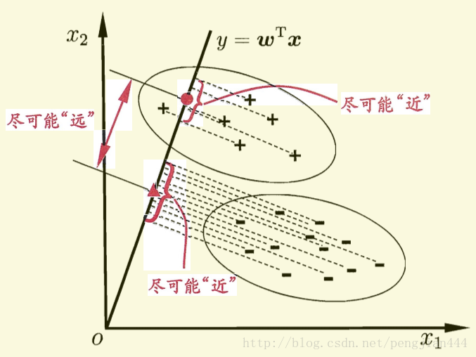
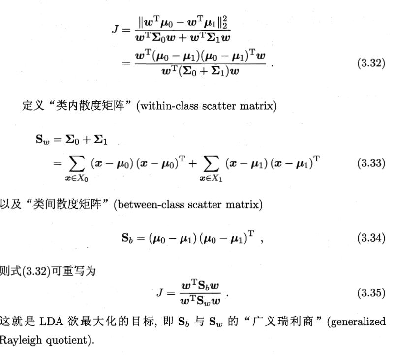
这样如果我们想要同类样列的投影点尽可能接近,可以让同类样列投影点的协方差尽可能小,即尽可能小;而欲使异类样列的投影点尽可能远离,可以让类中心之间的距离尽可能大,即尽可能大。同时结合两者我们可以得到欲最大化的目标:
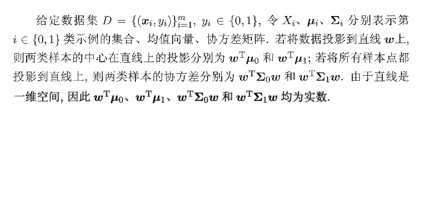
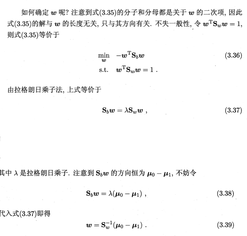
(本文图片截取自《机器学习》周志华)
有了上面的推理之后我们接下来就以DNA分类为例来实现一下Fisher线性判别。
数据准备
1
2
3
4
5
6
7
8
9
10
11
12
13
14
15
16
17
18
19
20
| from sklearn.cross_validation import train_test_split
dna_list = []
with open('dna2','r') as f:
dna_list = list(map(str.strip,f.readlines()))
f.close()
print(len(dna_list))
def generate_feature(seq):
for i in seq:
size = len(i)
yield [
chary.count(i,'a')/size,
chary.count(i,'t')/size,
chary.count(i,'c')/size,
chary.count(i,'g')/size]
X = np.array(list(generate_feature(dna_list)),dtype=float)
y = np.ones(20)
y[10:]=2
X_train, X_test, y_train, y_test = train_test_split(X[:20], y, test_size=0.1)
print(X_train,'\n',y_train)
|
输出结果:
40
[[ 0.2972973 0.13513514 0.17117117 0.3963964 ]
[ 0.35454545 0.5 0.04545455 0.1 ]
[ 0.42342342 0.28828829 0.10810811 0.18018018]
[ 0.35135135 0.12612613 0.12612613 0.3963964 ]
[ 0.27927928 0.18918919 0.16216216 0.36936937]
[ 0.21818182 0.56363636 0.14545455 0.07272727]
[ 0.20720721 0.15315315 0.20720721 0.43243243]
[ 0.3 0.5 0.08181818 0.11818182]
[ 0.2 0.56363636 0.17272727 0.06363636]
[ 0.27027027 0.06306306 0.21621622 0.45045045]
[ 0.32727273 0.5 0.02727273 0.14545455]
[ 0.23423423 0.10810811 0.23423423 0.42342342]
[ 0.29090909 0.64545455 0. 0.06363636]
[ 0.18181818 0.13636364 0.27272727 0.40909091]
[ 0.29090909 0.5 0.11818182 0.09090909]
[ 0.25454545 0.51818182 0.1 0.12727273]
[ 0.27433628 0.36283186 0.19469027 0.16814159]
[ 0.27027027 0.15315315 0.16216216 0.41441441]]
[ 1. 2. 1. 1. 1. 2. 1. 2. 2. 1. 2. 1. 2. 1. 2. 2. 2. 1.]
Fisher算法实现
1
2
3
4
5
6
7
8
9
10
11
12
13
14
15
16
17
18
19
20
21
22
23
24
25
26
27
| def cal_cov_and_avg(samples):
"""
给定一个类别的数据,计算协方差矩阵和平均向量
:param samples:
:return:
"""
u1 = np.mean(samples, axis=0)
cov_m = np.zeros((samples.shape[1], samples.shape[1]))
for s in samples:
t = s - u1
cov_m += t * t.reshape(4, 1)
return cov_m, u1
def fisher(c_1, c_2):
"""
fisher算法实现(请参考上面推导出来的公式,那个才是精华部分)
:param c_1:
:param c_2:
:return:
"""
cov_1, u1 = cal_cov_and_avg(c_1)
cov_2, u2 = cal_cov_and_avg(c_2)
s_w = cov_1 + cov_2
u, s, v = np.linalg.svd(s_w) # 奇异值分解
s_w_inv = np.dot(np.dot(v.T, np.linalg.inv(np.diag(s))), u.T)
return np.dot(s_w_inv, u1 - u2)
|
判别类型
1
2
3
4
5
6
7
8
9
10
11
12
13
14
15
16
17
18
19
20
21
22
23
24
25
26
27
28
29
30
| def judge(sample, w, c_1, c_2):
"""
true 属于1
false 属于2
:param sample:
:param w:
:param center_1:
:param center_2:
:return:
"""
u1 = np.mean(c_1, axis=0)
u2 = np.mean(c_2, axis=0)
center_1 = np.dot(w.T, u1)
center_2 = np.dot(w.T, u2)
pos = np.dot(w.T, sample)
return abs(pos - center_1) < abs(pos - center_2)
w = fisher(X_train[:10], X_train[10:20]) # 调用函数,得到参数w
pred = []
for i in range(20):
pred.append( 1 if judge(X[i], w, X_train[:10], X_train[10:20]) else 2) # 判断所属的类别
# evaluate accuracy
pred = np.array(pred)
print(y,pred)
print(metrics.accuracy_score(y, pred))
out = []
for i in range(20,40):
out.append( 1 if judge(X[i], w, X_train[:10], X_train[10:20]) else 2) # 判断所属的类别
print(out)
|
输出结果:
[ 1. 1. 1. 1. 1. 1. 1. 1. 1. 1. 2. 2. 2. 2. 2. 2. 2. 2.
2. 2.] [1 1 1 1 1 1 1 1 1 1 2 2 2 2 2 2 2 2 2 1]
0.95
[1, 1, 1, 1, 1, 1, 1, 2, 2, 1, 1, 2, 1, 1, 1, 1, 1, 2, 1, 1]
在这我们可以看出我们的Fisher算法在测试集中的误差率还算理想,误判率仅有5%。但是,我们可以看出其预测分类并不如其他KNN,SVM,等算法的预测效果。
最后,有关Fisher算法的介绍也就到此结束了!