机器学习之梯度下降

梯度下降(gradient descent)

是线性回归的一种(Linear Regression)，在Andrew Ng的machine learning前期课程中有着详细的讲解，首先给出一个关于课程中经典的例子:预测房屋的价格。

在上面的表格中，房间的个数以及房屋的面积都是输入变量而，价格就是我们要预测输出的值。其中，面积和房屋个数分别表示一个特征，我们在这将他们一起用X来表示。价格用Y来表示。同时表格的每一行表示成一个样本，具体表示为：$f: X_1=[24104,3] \to Y_1=400$。

那么我们具体的任务就可以概括成给定一个训练集合，学习出一个函数$f$，使得$f(x)$能够符合结果Y，或者说能够使得$f(x)$与Y的之间的误差最小。

我们可以用以下的式子来表达上述的关系：

$f(x) = \theta_1 x_1 + \theta_2 x_2 + \beta$

其中，$\theta 表示X映射成Y的权重，而x表示为各组特征。$
我们再分别用$x^{j},y^{j}来表示第J个样本$。这样我们就可以写出代价函数：

$J(\theta) = \frac {1}{2}\sum ^m_{i=0}(f_\theta(x^{i})-y^{(i)})^2$

然后我们要使得计算的结果无限接近真实值y的话，我们就要令得我们的代价函数（俗称的误差）最小化。要使得$J(\theta)$最小，即对$J(\theta)$进行求导操作，并使得其结果为0。

$\theta_j = \theta_j - \frac{\partial J(\theta)}{\partial \theta_j}$

当只有单个特征时，上式中的j表示系数（权重）的编号，右边的值赋给左边的变量后完成一次迭代过程。

而多个特征时，其迭代过程如下：

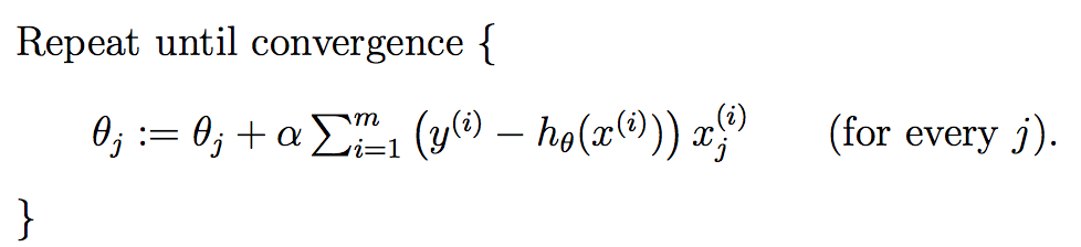
上式就是批梯度下降算法(batch gradient descent)，当上式收敛时则退出迭代，何为收敛，即前后两次迭代的值不再发生变化了。一般情况下，会设置一个具体的参数，当前后两次迭代差值小于该参数时候结束迭代。注意以下几点：

(1) a 即学习率（learning rate），决定的下降步伐，如果太小，则找到函数最小值的速度就很慢，如果太大，则可能会出现无法逼近最小值的现象；

(2) 初始点不同，获得的最小值也不同，因此梯度下降求得的只是局部最小值；

(3) 越接近最小值时，下降速度越慢；

(4) 计算批梯度下降算法时候，计算每一个θ值都需要遍历计算所有样本，当数据量的时候这是比较费时的计算。

批梯度下降算法的步骤可以归纳为以下几步：

(1)先确定向下一步的步伐大小，我们称为Learning rate ；

(2)任意给定一个初始值：θ向量，一般为0向量

(3)确定一个向下的方向，并向下走预先规定的步伐，并更新θ向量

(4)当下降的高度小于某个定义的值，则停止下降；

随机梯度下降算法

因为每次计算梯度都需要遍历所有的样本点。这是因为梯度是J(θ)的导数，而J(θ)是需要考虑所有样本的误差和 ，这个方法问题就是，扩展性问题，当样本点很大的时候，基本就没法算了。

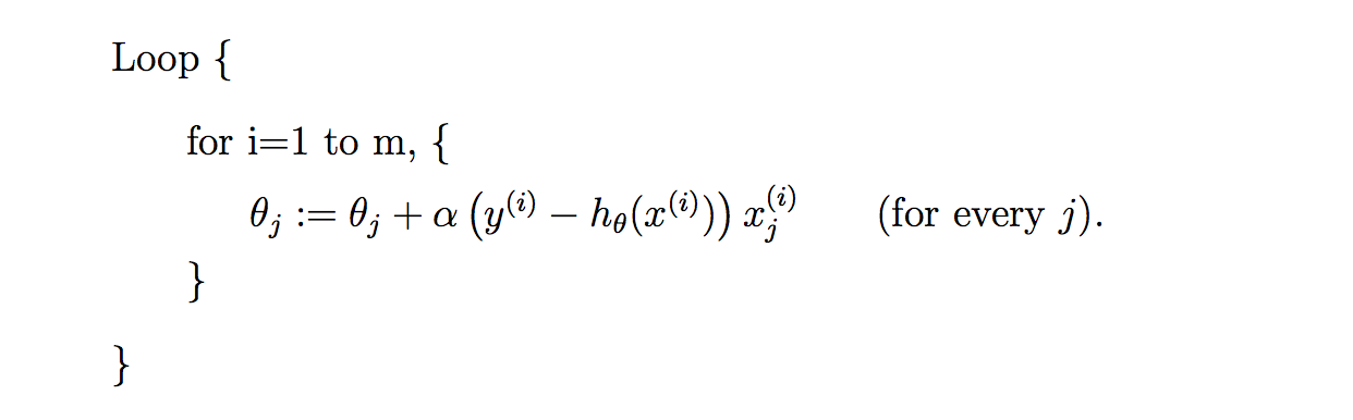
所以接下来又提出了随机梯度下降算法(stochastic gradient descent )。随机梯度下降算法，每次迭代只是考虑让该样本点的J(θ)趋向最小，而不管其他的样本点，这样算法会很快，但是收敛的过程会比较曲折，整体效果上，大多数时候它只能接近局部最优解，而无法真正达到局部最优解。所以适合用于较大训练集的例子。

其具体流程用公式表达如下：

代码实现

批梯度下降算法

1
2
3
4
5
6
7
8
9
10
11
12
13
14
15
16
17
18
19
20
21
22
23
24
25
26
27
28
29
30
31
32
33
34
35
36
37
38
39
40
41
42
43
44
45
46
47
48

#Training data set
#each element in x represents (x0,x1,x2)
x = [(1,0.,3) , (1,1.,3) ,(1,2.,3), (1,3.,2) , (1,4.,4)]
#y[i] is the output of y = theta0 * x[0] + theta1 * x[1] +theta2 * x[2]
y = [95.364,97.217205,75.195834,60.105519,49.342380]


epsilon = 0.000001
#learning rate
alpha = 0.001
diff = [0,0]
error1 = 0
error0 =0
m = len(x)

#init the parameters to zero
theta0 = 0
theta1 = 0
theta2 = 0
sum0 = 0
sum1 = 0
sum2 = 0
while True:

    #calculate the parameters
    for i in range(m):
        #begin batch gradient descent
        diff[0] = y[i]-( theta0 + theta1 * x[i][1] + theta2 * x[i][2] )
        sum0 = sum0 + alpha * diff[0]* x[i][0]
        sum1 = sum1 + alpha * diff[0]* x[i][1]
        sum2 = sum2 + alpha * diff[0]* x[i][2]
        #end  batch gradient descent
    theta0 = sum0;
    theta1 = sum1;
    theta2 = sum2;
    #calculate the cost function
    error1 = 0
    for lp in range(len(x)):
        error1 += ( y[i]-( theta0 + theta1 * x[i][1] + theta2 * x[i][2] ) )**2/2

    if abs(error1-error0) < epsilon:
        break
    else:
        error0 = error1

    print(' theta0 : %f, theta1 : %f, theta2 : %f, error1 : %f'%(theta0,theta1,theta2,error1))

print ('Done: theta0 : %f, theta1 : %f, theta2 : %f'%(theta0,theta1,theta2))

输出结果：
theta0 : 0.377225, theta1 : 0.625295, theta2 : 1.120912, error1 : 4405.869965
theta0 : 0.729497, theta1 : 1.193311, theta2 : 2.164098, error1 : 3094.652486
theta0 : 1.058680, theta1 : 1.708424, theta2 : 3.135362, error1 : 2089.261446
theta0 : 1.366497, theta1 : 2.174683, theta2 : 4.040070, error1 : 1335.974025
theta0 : 1.654541, theta1 : 2.595831, theta2 : 4.883186, error1 : 789.589683
theta0 : 1.924288, theta1 : 2.975327, theta2 : 5.669299, error1 : 412.137681
theta0 : 2.177098, theta1 : 3.316371, theta2 : 6.402654, error1 : 171.776368
theta0 : 2.414234, theta1 : 3.621921, theta2 : 7.087177, error1 : 41.856096
theta0 : 2.636861, theta1 : 3.894714, theta2 : 7.726499, error1 : 0.121739
theta0 : 2.846057, theta1 : 4.137277, theta2 : 8.323976, error1 : 28.034282
theta0 : 3.042819, theta1 : 4.351950, theta2 : 8.882714, error1 : 110.193963
……
theta0 : 98.101057, theta1 : -13.028753, theta2 : 1.133773, error1 : 3.473679
theta0 : 98.101058, theta1 : -13.028753, theta2 : 1.133773, error1 : 3.473678
theta0 : 98.101058, theta1 : -13.028753, theta2 : 1.133773, error1 : 3.473677
theta0 : 98.101059, theta1 : -13.028753, theta2 : 1.133773, error1 : 3.473676
theta0 : 98.101059, theta1 : -13.028753, theta2 : 1.133773, error1 : 3.473675
theta0 : 98.101060, theta1 : -13.028753, theta2 : 1.133772, error1 : 3.473674
theta0 : 98.101061, theta1 : -13.028753, theta2 : 1.133772, error1 : 3.473673
Done: theta0 : 98.101061, theta1 : -13.028753, theta2 : 1.133772

由上面的输出结果可以知道，梯度下降算法会在迭代一定次数后收敛于一个较少的损失值（即error）然而这并不是最优解而只是一个局部最小值（因为我们也可以从结果看到 theta0 : 2.636861, theta1 : 3.894714, theta2 : 7.726499, error1 : 0.121739，这项数据的最终error反而优于我们的最终解）。

随机梯度下降算法

1
2
3
4
5
6
7
8
9
10
11
12
13
14
15
16
17
18
19
20
21
22
23
24
25
26
27
28
29
30
31
32
33
34
35
36
37
38
39
40
41
42
43
44
45

#Training data set
#each element in x represents (x0,x1,x2)
x = [(1,0.,3) , (1,1.,3) ,(1,2.,3), (1,3.,2) , (1,4.,4)]
#y[i] is the output of y = theta0 * x[0] + theta1 * x[1] +theta2 * x[2]
y = [95.364,97.217205,75.195834,60.105519,49.342380]


epsilon = 0.0001
#learning rate
alpha = 0.01
diff = [0,0]
error1 = 0
error0 =0
m = len(x)


#init the parameters to zero
theta0 = 0
theta1 = 0
theta2 = 0

while True:

    #calculate the parameters
    for i in range(m):

        diff[0] = y[i]-( theta0 + theta1 * x[i][1] + theta2 * x[i][2] )

        theta0 = theta0 + alpha * diff[0]* x[i][0]
        theta1 = theta1 + alpha * diff[0]* x[i][1]
        theta2 = theta2 + alpha * diff[0]* x[i][2]

    #calculate the cost function
    error1 = 0
    for lp in range(len(x)):
        error1 += ( y[i]-( theta0 + theta1 * x[i][1] + theta2 * x[i][2] ) )**2/2

    if abs(error1-error0) < epsilon:
        break
    else:
        error0 = error1

    print (' theta0 : %f, theta1 : %f, theta2 : %f, error1 : %f'%(theta0,theta1,theta2,error1))

print ('Done: theta0 : %f, theta1 : %f, theta2 : %f'%(theta0,theta1,theta2))

输出结果：
theta0 : 2.782632, theta1 : 3.207850, theta2 : 7.998823, error1 : 7.508687
theta0 : 4.254302, theta1 : 3.809652, theta2 : 11.972218, error1 : 813.550287
theta0 : 5.154766, theta1 : 3.351648, theta2 : 14.188535, error1 : 1686.507256
theta0 : 5.800348, theta1 : 2.489862, theta2 : 15.617995, error1 : 2086.492788
theta0 : 6.326710, theta1 : 1.500854, theta2 : 16.676947, error1 : 2204.562407
theta0 : 6.792409, theta1 : 0.499552, theta2 : 17.545335, error1 : 2194.779569
theta0 : 7.223066, theta1 : -0.467855, theta2 : 18.302105, error1 : 2134.182794
theta0 : 7.630213, theta1 : -1.384304, theta2 : 18.982980, error1 : 2056.719790
……
theta0 : 97.986505, theta1 : -13.221170, theta2 : 1.257223, error1 : 1.553680
theta0 : 97.986620, theta1 : -13.221169, theta2 : 1.257186, error1 : 1.553579
theta0 : 97.986735, theta1 : -13.221167, theta2 : 1.257150, error1 : 1.553479
theta0 : 97.986849, theta1 : -13.221166, theta2 : 1.257113, error1 : 1.553379
theta0 : 97.986963, theta1 : -13.221165, theta2 : 1.257077, error1 : 1.553278
Done: theta0 : 97.987078, theta1 : -13.221163, theta2 : 1.257041

通过上述批梯度下降和随机梯度下降算法代码的对比，不难发现两者的区别：
随机梯度下降算法在迭代的时候，每迭代一个新的样本，就会更新一次所有的theta参数。
因此当样本数量很大时候，批梯度得做完所有样本的计算才能更新一次theta，从而花费的时间远大于随机梯度下降。但是随机梯度下降过早的结束了迭代，使得它获取的值只是接近局部最优解，而并非像批梯度下降算法那样就是局部最优解。